本文是“JavaScript
线性代数 ”教程的一部分。
在本文中,我们将介绍矩阵的大部分基本运算,依次是矩阵的加减法、矩阵的标量乘法、矩阵与矩阵的乘法、求转置矩阵,以及深入了解矩阵的行列式运算。本文将不会涉及逆矩阵、矩阵的秩等概念,将来再探讨它们。
矩阵的加减法
矩阵的加法 与减法 运算将接收两个矩阵作为输入,并输出一个新的矩阵。矩阵的加法和减法都是在分量级别上进行的,因此要进行加减的矩阵必须有着相同的维数。
为了避免重复编写加减法的代码,我们先创建一个可以接收运算函数的方法,这个方法将对两个矩阵的分量分别执行传入的某种运算。然后在加法、减法或者其它运算中直接调用它就行了:
1
2
3
4
5
6
7
8
9
10
11
12
13
14
15
16
17
18
19
20
21
22
23
24
25
26
27
28
29
class Matrix { componentWiseOperation (func, { rows } ) { const newRows = rows.map ((row, i ) => row.map ((element, j ) => func (this .rows [i][j], element)) ) return new Matrix (...newRows) } add (other ) { return this .componentWiseOperation ((a, b ) => a + b, other) } subtract (other ) { return this .componentWiseOperation ((a, b ) => a - b, other) } } const one = new Matrix ( [1 , 2 ], [3 , 4 ] ) const other = new Matrix ( [5 , 6 ], [7 , 8 ] ) console .log (one.add (other))console .log (other.subtract (one))
矩阵的标量乘法
矩阵的标量乘法与向量的缩放类似,就是将矩阵中的每个元素都乘上标量:
1
2
3
4
5
6
7
8
9
10
11
12
13
14
15
16
class Matrix { scaleBy (number ) { const newRows = this .rows .map (row => row.map (element => ) return new Matrix (...newRows) } } const matrix = new Matrix ( [2 , 3 ], [4 , 5 ] ) console .log (matrix.scaleBy (2 ))
矩阵乘法
当 A 、B
两个矩阵的维数是兼容 的时候,就能对这两个矩阵进行矩阵乘法。所谓维数兼容,指的是
A 的列数与 B 的行数相同。矩阵乘法
AB 就是对举证 A 的每一行行与矩阵
B 的每一列分别进行点积运算:
matrix-matrix multiplication
1
2
3
4
5
6
7
8
9
10
11
12
13
14
15
16
17
18
19
20
21
22
23
24
25
26
27
28
29
30
31
32
class Matrix { multiply (other ) { if (this .rows [0 ].length !== other.rows .length ) { throw new Error ('The number of columns of this matrix is not equal to the number of rows of the given matrix.' ) } const columns = other.columns () const newRows = this .rows .map (row => columns.map (column =>sum (row.map ((element, i ) => element * column[i]))) ) return new Matrix (...newRows) } } const one = new Matrix ( [3 , -4 ], [0 , -3 ], [6 , -2 ], [-1 , 1 ] ) const other = new Matrix ( [3 , 2 , -4 ], [4 , -3 , 5 ] ) console .log (one.multiply (other))
我们可以把矩阵乘法 AB 视为先后应用
A 和 B
两个线性变换矩阵。为了更好地理解这种概念,可以看一看我们的 linear-algebra-demo 。
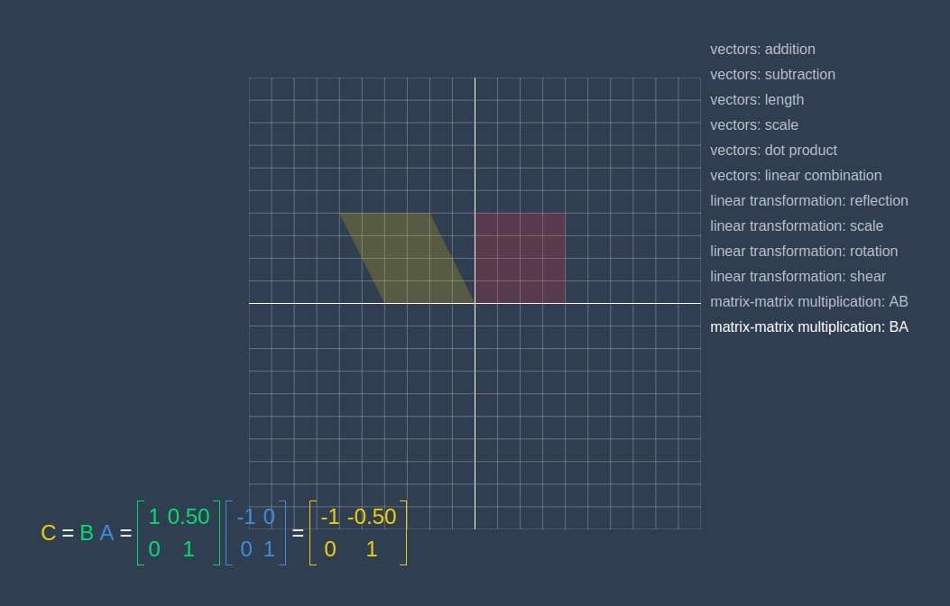
下图中黄色的部分就是对红色方块应用线性变换 C
的结果。而线性变换 C 就是矩阵乘法 AB
的结果,其中 A 是做相对于 y
轴进行反射的变换矩阵,B 是做剪切变换的矩阵。
先旋转再剪切变换
如果在矩阵乘法中调换 A 和 B
的顺序,我们会得到一个不同的结果,因为相当于先应用了 B
的剪切变换,再应用 A 的反射变换:
shear than rotate
转置
转置 矩阵 \(A^T\)
由公式 \(a^T_{ij}=a_{ji}\)
定义。换句话说,我们通过关于矩阵的对角线对其进行翻转来得到转置矩阵。需要注意的是,矩阵对角线上的元素不受转置运算影响。
1
2
3
4
5
6
7
8
9
10
11
12
13
14
15
16
17
18
19
20
21
class Matrix { transpose ( return new Matrix (...this .columns ()) } } const matrix = new Matrix ( [0 , 1 , 2 ], [3 , 4 , 5 ], [6 , 7 , 8 ], [9 , 10 , 11 ] ) console .log (matrix.transpose ())
行列式运算
矩阵的行列式 运算将计算矩阵中的所有系数,最后输出一个数字。准确地说,行列式可以描述一个由矩阵行构成的向量的相对几何指标(比如在欧式空间中的有向面积、体积等空间概念)。更准确地说,矩阵
A 的行列式相当于告诉你由 A
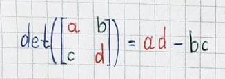
的行定义的方块的体积。\(2\times 2\)
矩阵的行列式运算如下所示:
det(2×2 matrix)
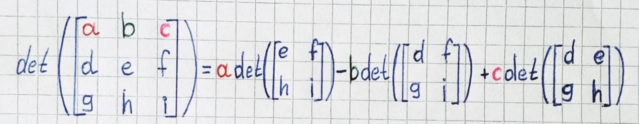
\(3\times 3\)
矩阵的行列式运算如下所示:
det(3×3 matrix)
我们的方法可以计算任意大小矩阵(只要其行列的数量相同)的行列式:
1
2
3
4
5
6
7
8
9
10
11
12
13
14
15
16
17
18
19
20
21
22
23
24
25
26
27
28
29
30
31
32
33
34
35
36
37
38
39
40
41
42
class Matrix { determinant ( if (this .rows .length !== this .rows [0 ].length ) { throw new Error ('Only matrices with the same number of rows and columns are supported.' ) } if (this .rows .length === 2 ) { return this .rows [0 ][0 ] * this .rows [1 ][1 ] - this .rows [0 ][1 ] * this .rows [1 ][0 ] } const parts = this .rows [0 ].map ((coef, index ) => { const matrixRows = this .rows .slice (1 ).map (row =>slice (0 , index), ...row.slice (index + 1 )]) const matrix = new Matrix (...matrixRows) const result = coef * matrix.determinant () return index % 2 === 0 ? result : -result }) return sum (parts) } } const matrix2 = new Matrix ( [ 0 , 3 ], [-2 , 1 ] ) console .log (matrix2.determinant ())const matrix3 = new Matrix ( [2 , -3 , 1 ], [2 , 0 , -1 ], [1 , 4 , 5 ] ) console .log (matrix3.determinant ())const matrix4 = new Matrix ( [3 , 0 , 2 , -1 ], [1 , 2 , 0 , -2 ], [4 , 0 , 6 , -3 ], [5 , 0 , 2 , 0 ] ) console .log (matrix4.determinant ())
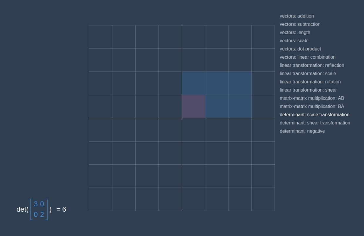
行列式可以告诉我们变换时对象被拉伸的程度。因此我们可以将其视为一个线性变换对区域改变的一个因素。为了更好地理解这个概念,请参考
linear-algebra-demo :
在下图中,我们可以看到对红色的 1×1
方形进行线性变换后得到了一个 3×2 的长方形,面积从
1 变为了
6 ,这个数字与线性变换矩阵的行列式值相同。
det(scale transformation)
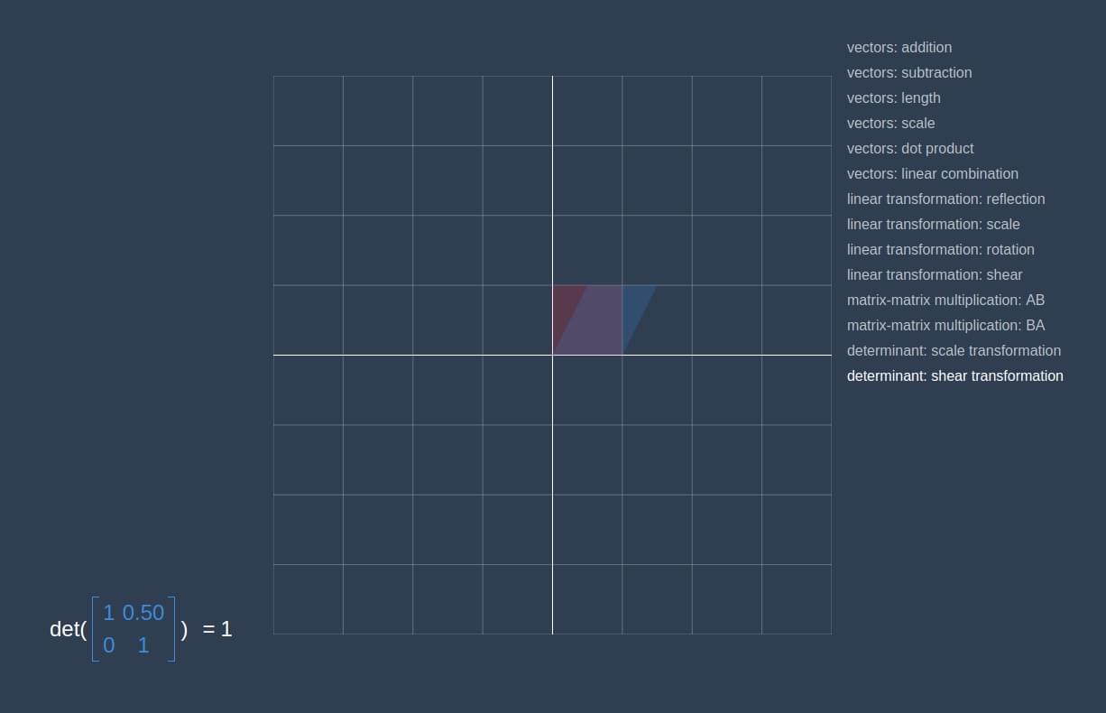
如果我们应用一个剪切变换,可以看到方形会变成一个面积不变的平行四边形。因此,剪切变换矩阵的行列式值等于
1:
det(shear transformation)
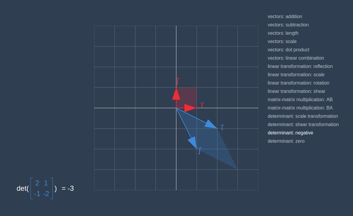
如果行列式的值是负数 ,则说明应用线性变换后,空间被反转了。比如在下图中,我们可以看到变换前
\(\hat{\jmath}\) 在 \(\hat{\imath}\) 的左边,而变换后 \(\hat{\jmath}\) 在 \(\hat{\imath}\) 的右边。
negative determinant
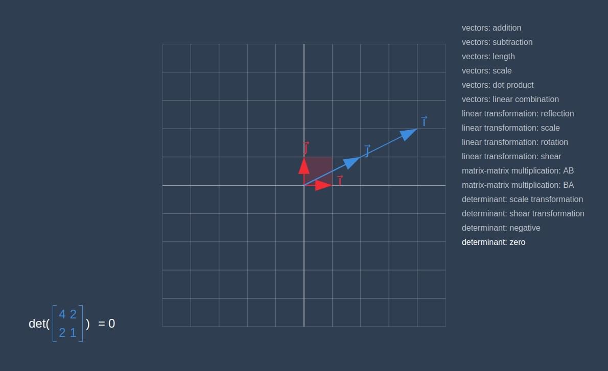
如果变换的行列式为
0 ,则表示它会将所有空间都压缩到一条线或一个点上。也就是说,计算一个给定矩阵的行列式是否为
0,可以判断这个矩阵对应的线性变换是否会将对象压缩到更小的维度去。
2D 中的 0 行列式
在三维空间里,行列式可以告诉你体积缩放了多少:
det(scale transformation) in
3D
变换行列式等于 0,意味着原来的空间会被完全压缩成体积为 0
的空间。如前文所说,如果在 2 维空间中变换的行列式为
0,则意味着变换的结果将空间压缩成了一条线或一个点;而在 3
维空间中变换的行列式为 0
意味着一个物体会被压扁成一个平面,如下图所示:
3D 中的 0 行列式